Tsukuba Challenge Dynamic Object Tracks Dataset

Tsukuba Challenge Dynamic Object Tracks Dataset

The MAD team presents the Tsukuba Challenge Dynamic Object Tracks Dataset which you can access on Github

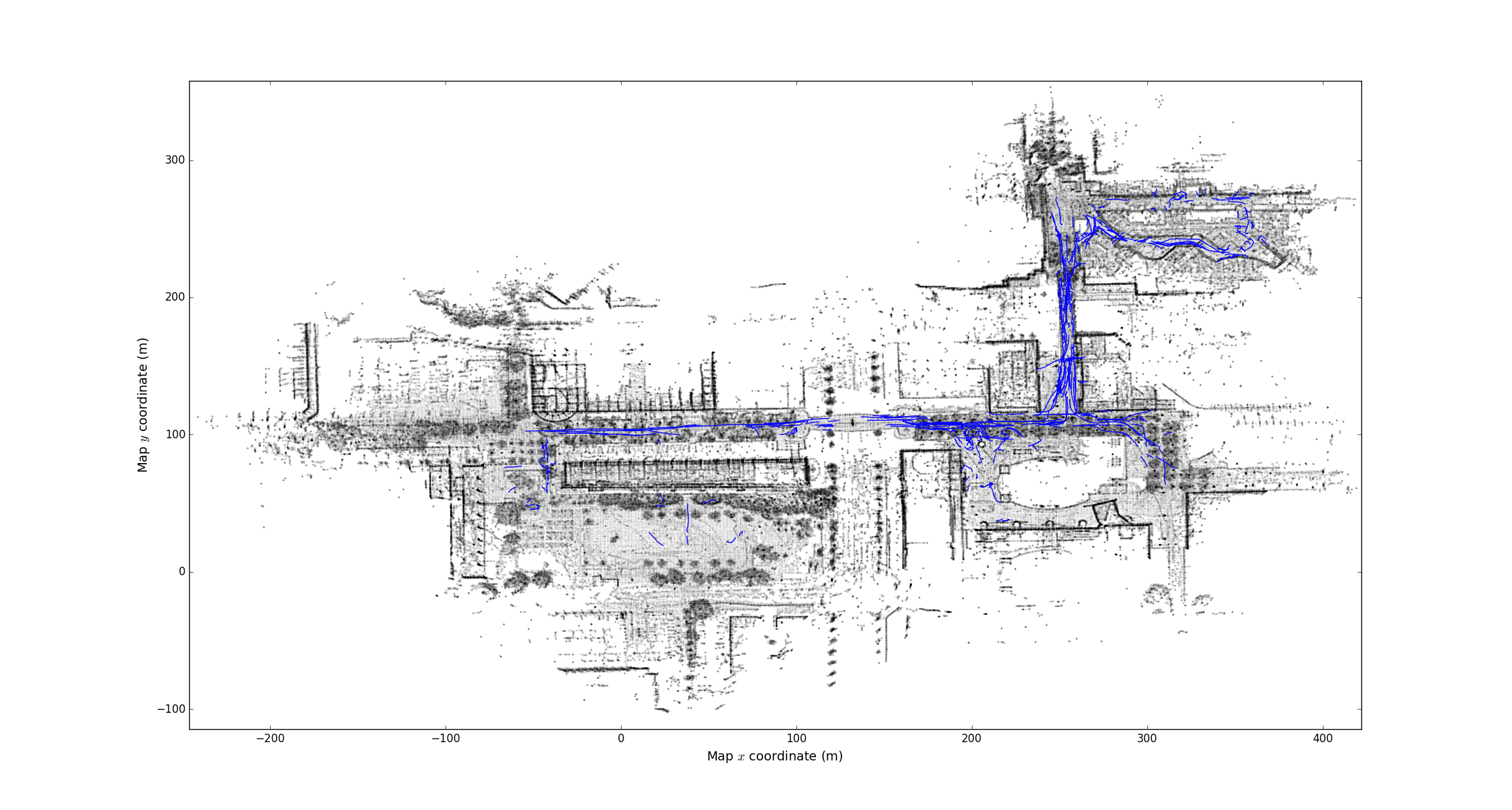
We collected 15 rosbags runs of the 2017 Tsukuba Challenge each of which covers the a distance of over 2 kilometers. The following is a top view of the course, where our trajectory is in red and approximate traversable area is in green: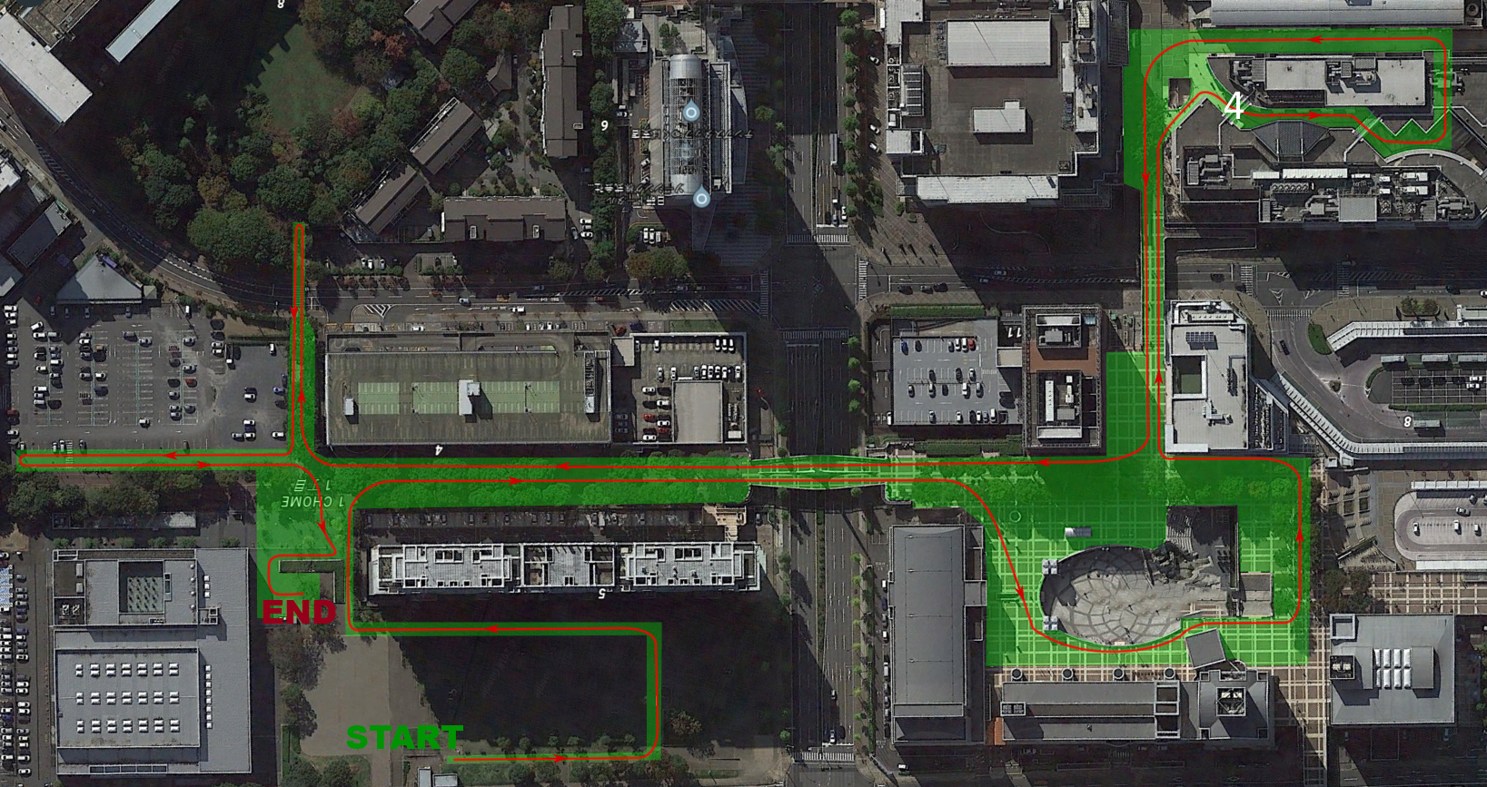 

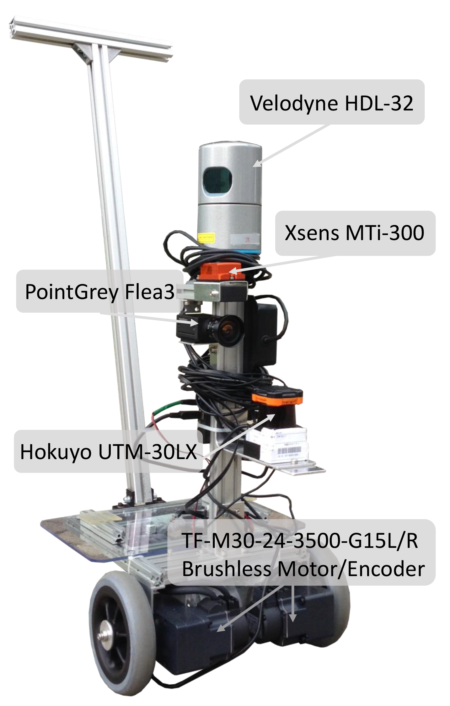We use the MinBot to collect this data, which you can see below. It is a manually operated data collection platform, equipped with many sensors: Velodyne HDL-32 3D lidar, Hokuyo UTM-30LX 2D lidar, PointGrey Flea3 monocular camera, Xsens MTi-300 intertial motion unit (IMU) as well as wheel encoders.

Though we logged information for all sensors, note that for this research we use the Velodyne HDL-32 3D lidar alongside wheel odometry for localization, and only 3D lidar for dynamic object detection and tracking.

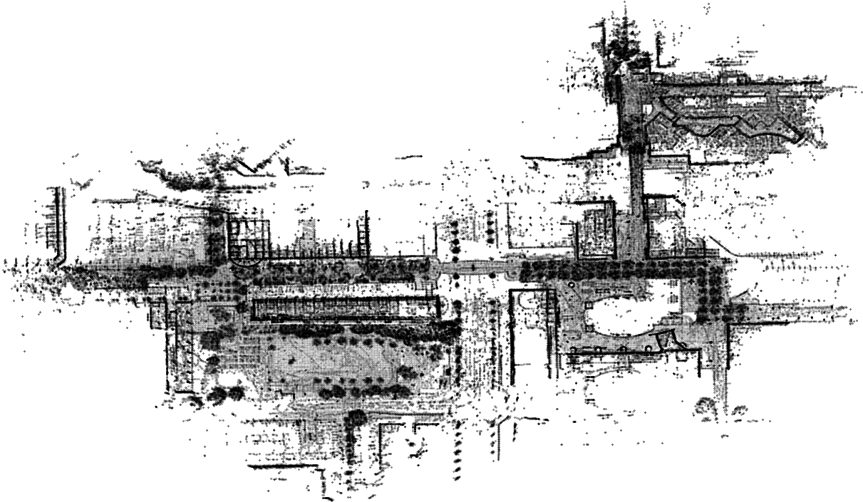
We use Autoware’s NDT Mapping and Localization tool to create a 3D Lidar Map of the environment which we use, alongside odometry, to localize. Then, using multiple runs of the environment, we use Octomap to create a 3D occupancy grid of the environment’s static background. The final map of the environment can be seen below.

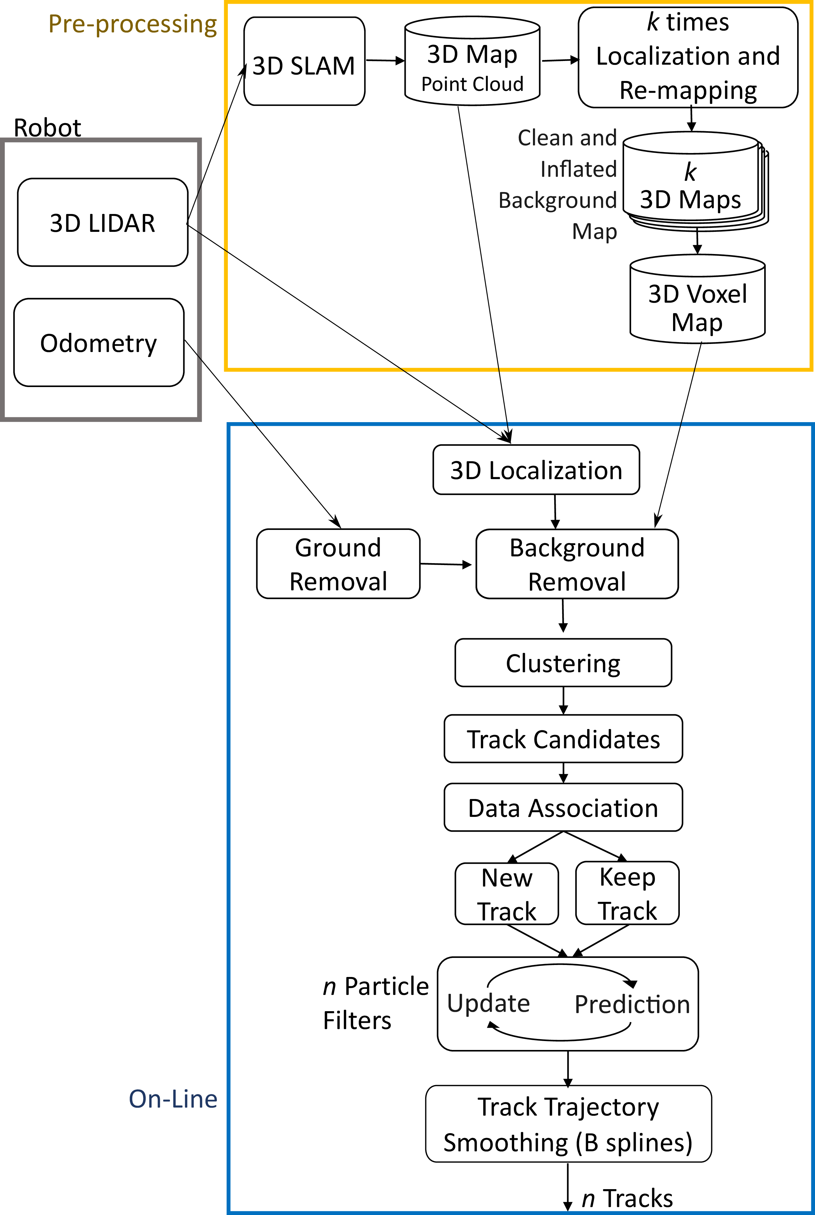
With localization capabilities and a static background map, we can now perform the dynamic object detection and tracking from the Lidar data:

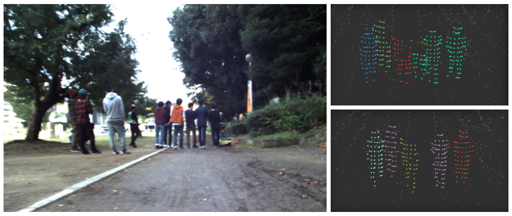
Points remaining after ground and background removal are then clustered using PCL’s Euclidean Clustering. This was often insufficient as pedestrians naturally move in clusters so several people are often grouped as one. To solve this issue we performed multiple maxima (heads) iterative sub-clustering. This is an important step as illustrated below. A group of 6 people block the road. Due to the point of view of the 3D Lidar, three people on the right are grouped into one cluster, one of which is heavily occluded. After sub-clustering, we have two clear people, with the third being rejected since cluster size is not big enough to truly determine whether this is a person.

The occluded person may eventually come into view and be added into our list of tracked objects. At each lidar frame, we look for new objects, perform data association and track existing objects using a particle filter. We also interpolate the trajectories of objects using b-spline, both to predict future position and to smooth out existing trajectories which can be noisy due to lidar noise.

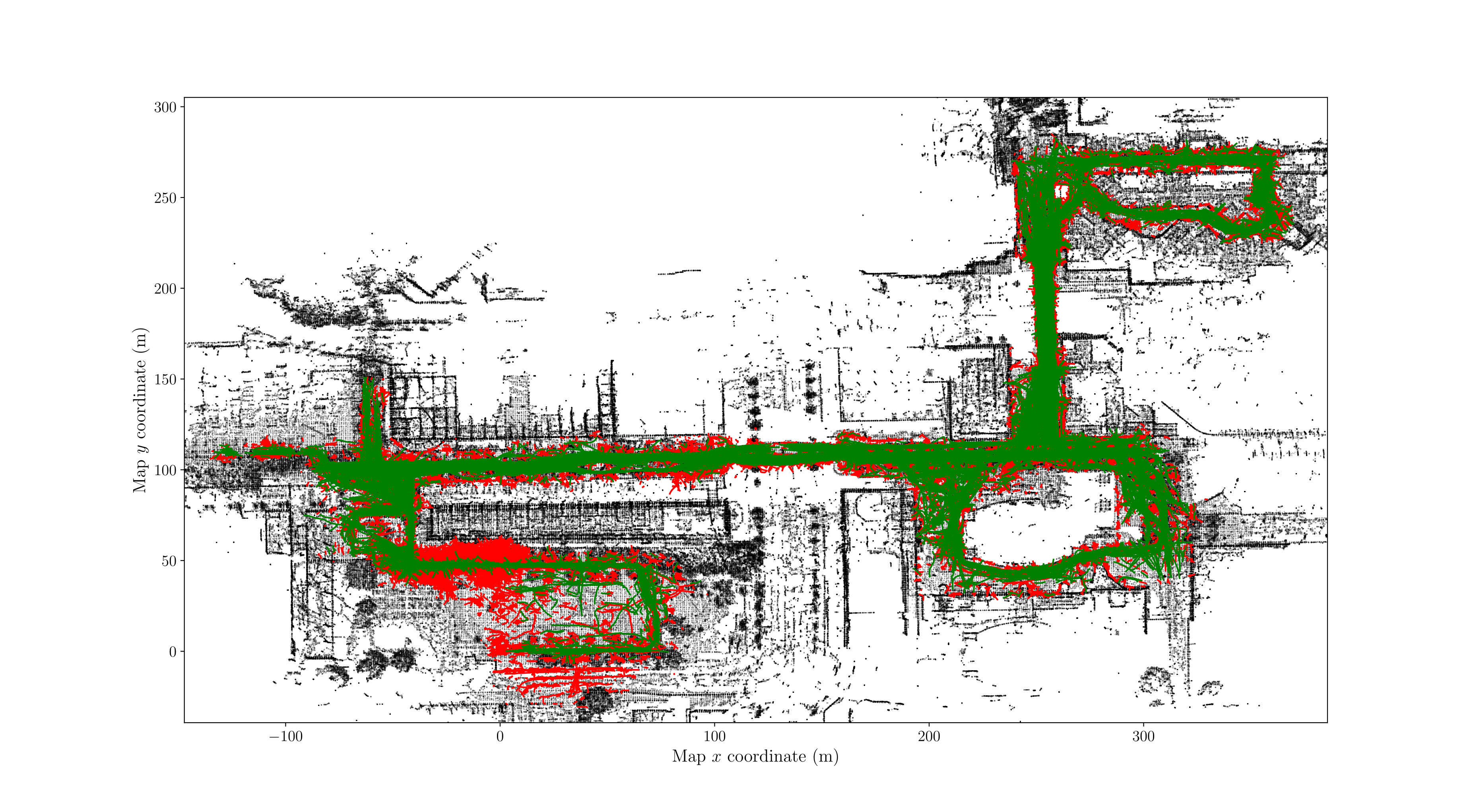
Also due to Lidar noise or poor localization, we often pick up background as dynamic objects for few milliseconds. This is especially problematic in areas like the Tsukuba Tent Area, which has a lot of shifting background. We can however filter out these false positives fairly easily by checking some statistics of the trajectories. We filter out trajectories with unnatural speed or rotational velocity, as well as objects that were tracked for very short distance of amount of time. Below, you can see all good trajectories in green, and all filtered our trajectories in red:

After filtering, we have a sanitized dataset of dynamic objects with the following information:

• Map of the Tsukuba Environment: 3D point cloud map and 2D occupancy grid map of the Tsukuba challenge environment.
• Robot Trajectory: position of the robot inside the map at each timestamp. Dynamic Object Locations: 2D and 3D locations of dynamic objects, with object ID and timestamp, localized in a global coordinate frame.
• 2D Smoothed Trajectories: b-spline-derived smooth trajectories.
• Velocity and Heading: derived velocity and heading from the smooth trajectory for each dynamic objects.
• Bounding Box: 3D bounding boxes and centroid location of each object.
• Object Point Clouds: 3D points inside each objects bounding box.

The data is currently available on Google Drive.

Data analysis tools

In this section I’ll go over the Meidai Data Tools module for the 2017 Tsukuba Challenge Dataset.

This python module includes two packages:

• dict_tools: some tools demonstrating how to load the data from the dictionary and how the dictionary was created from the raw text files.
• vis_tools: tools at your convenience to visualize the data.

First, you need to install the module, simply: python setup.py install

The module has a few requirements that are not included by default in python:

• numpy
• matplotlib
• seaborn

dict_tools

The dictionary tools module gives you functions and examples to load the Tsukuba Challenge data which is store in python dictionaries inside of pickle files. loader.py contains all the information you need to access the data inside the pickle ‘.pk1’ files:

The pickle file holds a dictionary with 4 keys, each in turn holding a dictionary with the trajectory ID as key

• 'raw_tracks' : raw trajectory data
• 'tracks' : b-spline smoothed trajectories
• 'filtered' : b-spline trajectories filtered for false positives with derived heading, velocity and rotational velocity (see paper or create_dict for filtering details)
• 'pointclouds' : segmented pointclouds for each object

Some illustrative code snippets: (or any other of the above 4 keys) returns all track IDs as keys in that dictionary. print dataset['raw_tracks'].keys() is also a dictionary. print dataset['pointclouds'][track_ID].keys() returns all the timestamps at which the dataset was observed, as keys to that dictionary.

The data is stored in numpy ndarrays of dtype=float32:

• map_data is a Nx3 matrix of points, centroids for the voxel grid
• dataset['raw_tracks'][track_ID] : N x 7 [timestamp, position_x, position_y, position_z, orientation_w, variance_x, variance_y] approximating the 2D particle filter distrubution as a gaussian, we get the above variance
• dataset['tracks'][trackID] : N x 3 [obstime, positionx, positiony]
• dataset['filtered'] : N x 7, [timestamp. position_x, position_y, heading, velocity_x, velocity_y, rotation_w] heading is from +x-axis, ccw [-pi, pi]
• dataset['pointclouds'][trackID][timestamp] : K x 3, [x, y, z]

You can run the loader through command line: python loader.py path/to/dataset.pk1 path/to/map.txt but you can also run it in your favorite IDE and change the dataset_file and map_file

vis_tools

These scripts show how you can plot various aspects of the data. All run the same way as the loader.

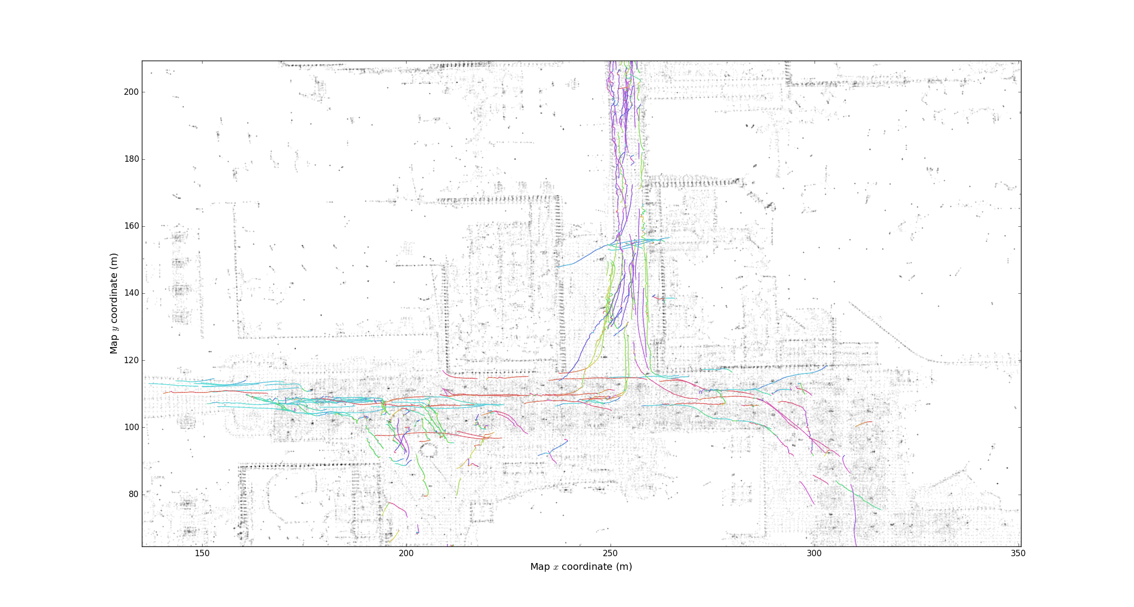
• plot_tracks.py: plots the track as simple lines with the map.

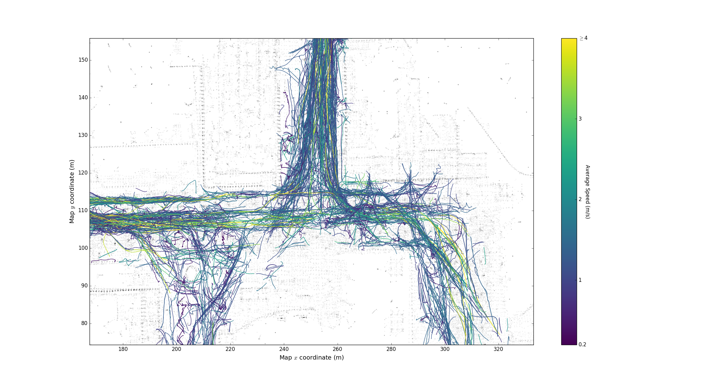
• plot_velocity.py: plots the track colored by average velocity. You can set the minimum and maximum velocity of the colormap inside the script.

• plot_headings.py: plots the trajectories by current settings, changing color every few timesteps, controlled by the stride parameter.

• plot_pointclouds.py: plots segmented pointclouds, for each track ID then each timestep. The script plots the next timestep when you close the window. If the color of the points change, the track_ID changed.
• plot_pointcloud_seq.py: plots segmented pointclouds, for each track ID then each timestep like the previous script, but keeps around a few (up to 4) timesteps of point with progressively stronger transparent. The current timestep has no alpha and black border.